Lab 2: Radiometric and Atmospheric Correction

Introduction

The goal of this lab was to practice correcting atmospheric interference of remotely sensed images. Using ERDAS Imagine, ArcMap, and Microsoft Excel, a series of multispectral images and the various spectral bands they are comprised of were corrected to represent true surface reflectance of land features.

Methods

Part 1: Absolute atmospheric correction using Empirical Line Calibration (ELC)

In the first part of this lab, a multispectral image of the greater Eau Claire area taken in 2011 by the Landsat 5 Thematic Mapper (TM) satellite, was corrected to represent at-surface spectral profiles of land features. By referencing libraries of typical spectral profiles of various surfaces, the Spectral Analysis Workstation tool was used to convert brightness values of surface features collected by the sensor, to a more typical set of brightness values for those surface features at ground level.

Figure 1: Select Atmospheric Adjustment tool in Spectral Analysis Workstation window.

Figure 2: Adjusting spectral profiles of surface features with the Atmospheric Adjustment tool in the Spectral Analysis Workstation model in ERDAS Imagine.

In Figure 2, the original multispectral image was brought into the Atmospheric Adjustment tool and sample points were added to the image over various surface features (asphalt, coniferous forest, agricultural land, aluminum roof, and lake water). The typical spectral profiles were added to the sample profiles using the ASTER and USGS V4 spectral libraries. In the "Spectrum Plot for Sample #5" window, the blue line represents the spectral profile of the sample point and the black line represents the spectral profile of tap water (the closest substitute for the true surface reflectance of Lake Wissota on the day of image capture).

After a sample point was collected for each surface feature, the tool was ran and generated an output image that was used to compare the spectral profiles of surface features after atmospheric correction with those of the original image (see Results).

Part II: Absolute atmospheric correction using enhanced image-based Dark Object Subtraction (DOS)

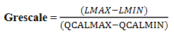
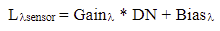
In the second part of this lab, a multispectral image of the greater Eau Claire area taken in 2011 by the same sensor as the image used in Part 1 (Landsat 5 TM) was corrected for atmospheric interference using the DOS method. This method converts the brightness values (spectral reflectance) of the original image to at-sensor spectral reflectance values, then to true surface reflectance values by using sensor gain and offset, solar irradiance and zenith angle, atmospheric scattering and absorption, and path radiance in two subsequent equations (Figures 3 and 4).

Figure 3: At-sensor spectral radiance equation.

In Figure 3, the LMAX and LMIN values represent the highest and lowest at-sensor spectral radiance values located in the sensor's metadata. The Qcal, Qcal Max, and Qcal Min values represent the layer image, and the highest and lowest calibrated pixel values in the image, also found in the sensor's metadata.

Figure 4: True surface reflectance equation.

In Figure 4, the π value is 3.14159 and the D2 value represents the distance between the earth and sun on the day of image capture. The Lλ and Lλhaze values represent the output image from the first equation (at-sensor spectral radiance image) and the path radiance (Figure 5). The TAUv, Esunλ, COS Θs, and TAUz values represent the atmospheric transmittance from the ground to the sensor (1), the mean atmospheric spectral irradiance for the particular image band being corrected (given by instructor), the cosine of sun zenith angle (given by instructor), and the atmospheric transmittance from the ground to the sun (given by instructor, not required for bands 5 and 7).

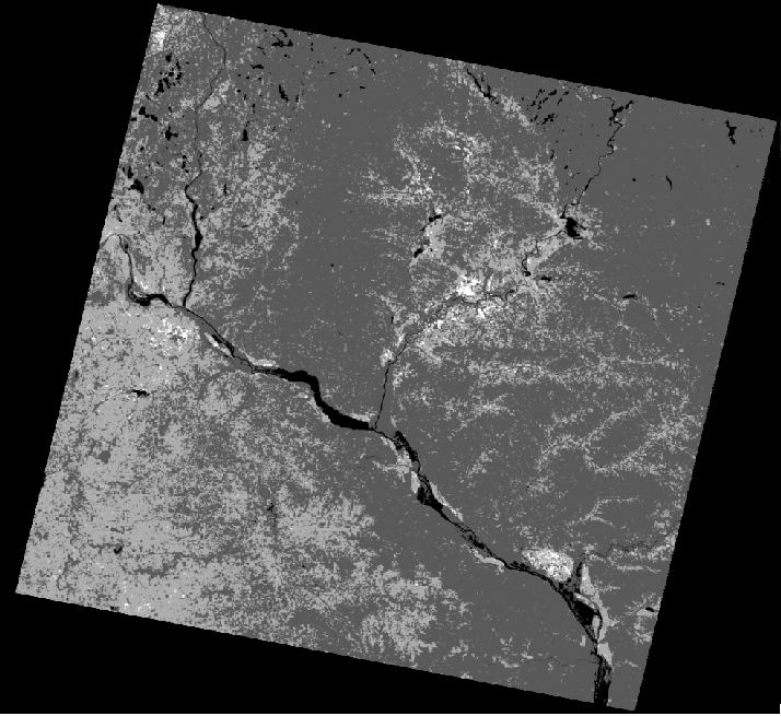
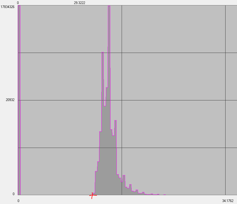
Figure 5: Visualization of path radiance value for band 1 (located in layer histogram).

To maximize the efficiency of calculating the two-part equation for all 6 bands, a model containing all inputs, outputs, and equations was created to sequentially generate at-sensor radiance and true surface reflectance images for each band (Figure 6).

Figure 6: Model that generates at-sensor radiance and true surface reflectance images of all 6 bands.

In Figure 6, the highlighted labels represent the original image, at-sensor radiance image (first output), and true surface reflectance image (final output) of the blue band (band 1).

Once all of the true surface reflectance images were created, a Layer Stack operation was performed to generate a multispectral image containing true surface reflectance brightness values.

Figure 7: Running a Layer Stack model on the true surface reflectance individual band images.

Part III: Relative atmospheric correction using Multidate Image Normalization

In the third and final part of this lab, two images capturing the same greater Chicago area from two different time signatures were combined using the Spectral Profile Viewer to collect the spectral profiles of various surface features in the images. Then, the mean brightness values of each spectral band in both images were brought into Microsoft Excel to generate a linear regression model. The values of which were then used to normalize the spectral signatures of the surface features between the two image dates.

First, the 2000 and 2009 images were brought into separate viewers in ERDAS Imagine. Then, the Spectral Profile Viewer was used to collect six samples in Lake Michigan, five samples of urban and built-up areas, and four samples of on-land water bodies (Figures 8 and 9).

Figure 8: Various surface feature sample point locations.

Figure 9: Spectral Profiles of sample points.

Once the sample points were collected, the Spectral Profile Viewer window was used to view the tabular data of the mean pixel values for each band in each image. This data was transferred to Microsoft Excel to generate a scatter plot and linear regression model (Figure 10).

Figure 10: Tabular data and Linear Regression Model of mean pixel values for both images.

Next, the linear equation and R-squared values were used in Model Builder to correct the image reflectance differences for each image band.

Figure 11: Equation used for normalizing at-sensor radiance of the image bands.

In Figure 11, the Gainλ represents the regression coefficient (R-squared value in Figure 10), the DN represents the input image (in this case, the individual image bands of the 2009 image), and the Biasλ represents the linear regression intercept (-2.6739 in the linear regression equation in Figure 10). The model containing all six input image bands, equations, and normalized output image bands is shown in Figure 12.

Figure 12: Model for normalizing the individual image bands of the 2009 Chicago multispectral image.

Once the model was run and the normalized output images were created, the Layer Stack operation in ERDAS Imagine was used to create a normalized multispectral image of the greater Chicago area.

Figure 13: Layer stacking the individually corrected at-sensor spectral radiance band images. 

Results

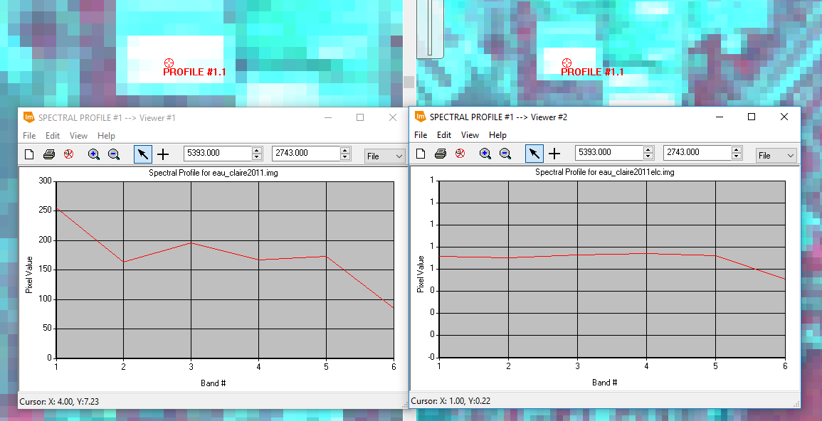
Figure 14: Comparing spectral profile of aluminum roof for original image (left) and corrected image (right).

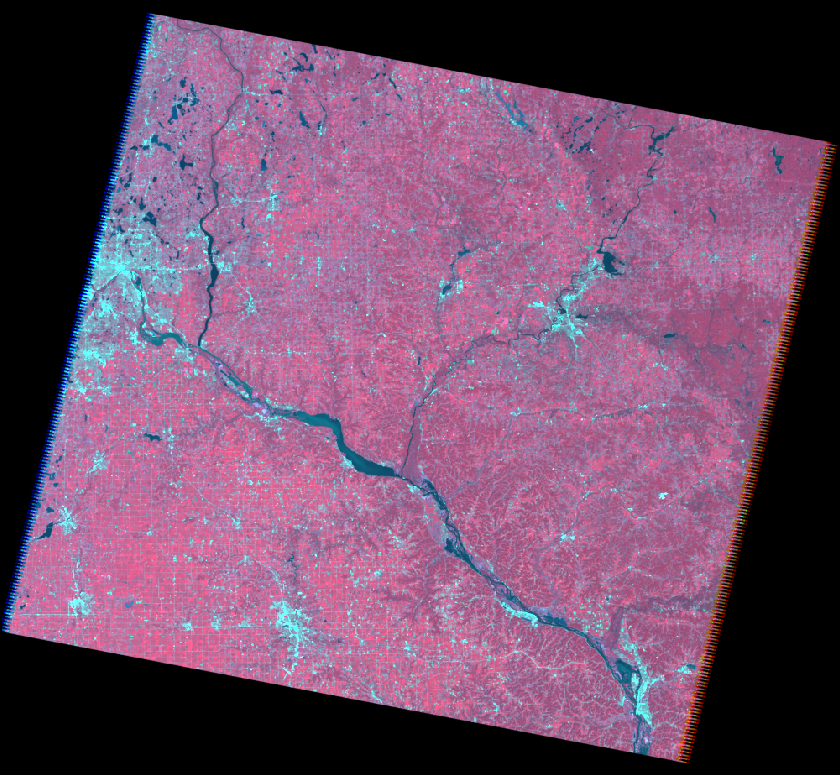
Figure 15: Multispectral composite for DOS method.

Figure 16: Multispectral composite for Multidate Image Normalization method.

After looking at the results, it is clear that any atmospheric correction performed on the images isn't incredibly obvious by just looking at the resulting images. When the spectral profiles of the surface features in the images are studied, however, the differences become much more distinguishable.

Conclusion

For part one, the empirical line calibration method turned out to be a decent method for adjusting for atmospheric interference. Although using the general spectral libraries doesn't provide the most accurate spectral correction, it does reduce the atmospheric windows that are a result of atmospheric interference and, in that regard, are helpful in getting a glimpse of surface reflectance.

For part two, the dark object subtraction method turned out to be the most accurate form of adjusting for atmospheric interference. By using constants from the satellite itself, values from the image data, and other mathematical constants (ie. pi), the calculations performed on each spectral band to eliminate the interference of the atmosphere generated particularly accurate image bands that were then stacked to produce an accurate multispectral image also.

For part three, the multidate image normalization method would've been a great method for eliminating variance in atmospheric conditions between two dates if the procedure was performed properly. Having misunderstood the instructions, the linear regression model used to calibrate the image bands was incorrect. Only 7 mean brightness values were used for each image and only one linear regression model was produced when, in actuality, 10 mean brightness values should've been used for each image band to generate 6 linear regression models. The lack of effectiveness in this effort was shown when studying the spectral profiles of the original and "corrected" images. It was even visible in the resulting image, as it appears very bright and has low spatial resolution.

Overall, it was very interesting to see the difference atmospheric correction had on the spectral profiles of surface features and helped reiterate the importance of atmospheric correction. The methods used in this lab have their differences in quality, but also have their particular uses and functions. For instance, if an image analyst only needs a rough idea of surface feature profiles and/or quick classification, the empirical line calibration method could suffice instead of the time-intensive, but more accurate method of dark object subtraction.

Sources

Data provided by Dr. Cyril Wilson and Landsat 5 TM
Image processing and atmospheric correction performed in ERDAS Imagine and ArcMap

Lab 1: Surface Temperature Extraction from Thermal Remote Sensing Data

Introduction

The purpose of this lab was to become familiar with the process of extracting radiant temperatures from surface features using thermal remote sensing images. Using ERDAS Imagine, an image processing software, multiple images were used in accordance with metadata to calculate the temperature of surface features from brightness values recorded at the sensor.

Methods

Part I: Visual Identification of Relative Variations in Land Surface Temperature

In part one of this lab, the goal was to identify surface features in a similar way to multispectral image interpretation, in that two thermal images captured by the Landsat ETM+ were observed and differences in the tonal quality were noted. The 61st band (one of two thermal sprectral bands on the Landsat ETM+) represents a high-gain thermal image and the 62nd band (the other thermal spectral band on the Landsat ETM+) represents a low-gain thermal image.

The low-gain image (band 62) was then compared to a multispectral reflective image captured from the same satellite, Landsat ETM+.

Finally, the sensor that collected information for the low-gain image was studied to understand what the spatial resolution of the image is when collected by the sensor (60 meters) and speculate as to why the difference in spatial resolution between the low-gain thermal image and multispectral reflective image is so great (see Results section).

Part II: Section I. Conversion of Digital Numbers to At-Satellite Radiance

In part two of this lab, a model was created to transform the brightness values (visual representation of tone stored as bits) of the low-gain image from part one into the radiance values that were collected by the thermal sensor. To do this, an equation was used that converts the digital numbers (bits) of the image to at-sensor spectral radiance (shown in figure 1).

Figure 1: At-sensor spectral radiance equation, where: grescale represents rescaled gain; brescale represents rescaled bias; and DN represents the digital numbers of the image band.

To find the grescale value, the following equation was used:

Figure 2: Grescale equation, where: L-Min and L-Max represent the lowest and highest radiance values collected at-sensor (located in metadata); and QCalMin and QCalMax represent the lowest and highest pixel values (bits) of the image.

After the grescale was calculated, using information stored in the image metadata, the input values for the function in Figure 1 were used in model builder (shown in figure 3).

Figure 3: Calculating at-sensor spectral radiance using model builder in ERDAS Imagine.

In Figure 3, the input image is the low-gain thermal band, the function is shown in the function definition window, and the output image was given a name and storage location. The output image (see Results section) would contain the at-sensor spectral radiance values for the image instead of brightness values stored in bits.
 
Part II: Section II. Conversion of At-Satellite Radiance to Blackbody Surface Temperature

Using the output image from part two: section one, the objective for this section was to extract the radiant temperatures of the surface features in the image. Although the surface radiance temperatures collected in this section are not the true kinetic temperatures of the surface features in the image, finding these values are the next necessary steps to finding the true kinetic temperatures of the surface features.

This was done by using the following formula:

Figure 4: Blackbody radiance temperatures equation, where: K1 and K2 are pre-launch calibration constants; and Lλ represents the at-sensor spectral radiance image.

The K1 and K2 values were obtained from the image metadata. Along with the rest of the inputs, the function was calculated using another model (shown in figure 5).

Figure 5: Calculating blackbody radiance temperatures (°K).

The input image in Figure 5 was the at-sensor spectral radiance image generated in section one of part two, the function is shown in the function definition window, and the output image was given a name and storage location. The output image (see Results section) would contain blackbody radiance temperatures in °K.

Part III: Calculation of Land Surface Temperature from TM Image

Using a thermal image band from a different satellite (Landsat TM), similar methods from part two of this lab were used, with the exception of combing the two steps into one (note: the models shown in figure 6 and 7 are one function, both function definition windows could not be displayed synonymously and therefore had to be split into two images), and with the appropriate constants and inputs for the image (shown in figures 6 and 7).

Figure 6: Calculating at-sensor spectral radiance for the Landsat TM thermal image band.

In Figure 6, the input image was the thermal image band from Landsat TM, the function is shown in the Function Definition window, and the output image was saved as a temporary raster.

Figure 7: Calculating blackbody radiance temperatures of the Landsat TM thermal image band (°K).

In Figure 7, the input image was the at-sensor spectral radiance temporary raster, the function is shown in the Function Definition window, and the output image was given a name and storage location.

Part IV: Calculation of Land Surface Temperature from Landsat 8 Image

In the fourth part of this lab, similar steps to part three were used with a different satellite image (acquired from Landsat 8) and respective constants/input values; only this time, an area of interest (AOI) shapefile was used to subset the image (see figures 8 and 9). Again, the following two images are from the same function.

Figure 8: Calculating at-sensor spectral radiance for the Landsat 8 thermal image band.

The input image in Figure 8 is the thermal image band from Landsat 8, the function is shown in the Function Definition window, and the output image was given a name and storage location.

Figure 9: Calculating blackbody radiance temperatures of the Landsat 8 thermal image band (°K).

The input image in Figure 9 was the output image in Figure 8, the function is shown in the Function Definition window, and the output image was saved as a temporary raster. The temporary raster was then brought into ArcMap, classified, and used to create a map of the surface feature radiance temperatures of the AOI (see Results section).

Results

Part I
The low-gain image has a greater contrast than the high-gain. The lowest brightness values (BV) in the high-gain image are lower than those in the low-gain image. The range of BV in the low-gain image is greater than those in the high-gain image as well.

Part II: Section I

Figure 10: At-sensor spectral radiance for Landsat ETM+ thermal image band.

Part II: Section II

Figure 11: Blackbody radiance temperature for Landsat ETM+ thermal image band.

Part III

Figure 12: Blackbody radiance temperature for Landsat TM thermal image band.

Part IV

Figure 13: Blackbody radiance temperatures for Landsat 8 thermal image band.

Conclusion

Upon completion of this lab, three different thermal images from three different satellites captured different results for blackbody radiance temperatures. Due to the time differences between the images, the radiance temperatures of various surface features are unique to each image output. To distinguish these differences, the resulting images were brought into ArcMap and the identify tool was used to determine the radiant temperatures of central Lake Wissota in each image. The temperature difference of Lake Wissota between 2000 and 2011 was 262.8°K, or 13.4°F.

Overall, this lab proved how important metadata is to thermal remote sensing, how effective and easy model builder is to use for converting image values from bits to blackbody radiance temperatures, and how temporal resolution affects temperatures of remotely sensed thermal images.

Sources

Data provided by Landsat 8 satellite, U.S. Census Bureau, and Dr. Cyril Wilson
Processing and cartography completed in ERDAS Imagine and ArcMap educational software packages