Lab 1: Surface Temperature Extraction from Thermal Remote Sensing Data

Introduction

The purpose of this lab was to become familiar with the process of extracting radiant temperatures from surface features using thermal remote sensing images. Using ERDAS Imagine, an image processing software, multiple images were used in accordance with metadata to calculate the temperature of surface features from brightness values recorded at the sensor.

Methods

Part I: Visual Identification of Relative Variations in Land Surface Temperature

In part one of this lab, the goal was to identify surface features in a similar way to multispectral image interpretation, in that two thermal images captured by the Landsat ETM+ were observed and differences in the tonal quality were noted. The 61st band (one of two thermal sprectral bands on the Landsat ETM+) represents a high-gain thermal image and the 62nd band (the other thermal spectral band on the Landsat ETM+) represents a low-gain thermal image.

The low-gain image (band 62) was then compared to a multispectral reflective image captured from the same satellite, Landsat ETM+.

Finally, the sensor that collected information for the low-gain image was studied to understand what the spatial resolution of the image is when collected by the sensor (60 meters) and speculate as to why the difference in spatial resolution between the low-gain thermal image and multispectral reflective image is so great (see Results section).

Part II: Section I. Conversion of Digital Numbers to At-Satellite Radiance

In part two of this lab, a model was created to transform the brightness values (visual representation of tone stored as bits) of the low-gain image from part one into the radiance values that were collected by the thermal sensor. To do this, an equation was used that converts the digital numbers (bits) of the image to at-sensor spectral radiance (shown in figure 1).

Figure 1: At-sensor spectral radiance equation, where: grescale represents rescaled gain; brescale represents rescaled bias; and DN represents the digital numbers of the image band.

To find the grescale value, the following equation was used:

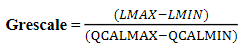Figure 2: Grescale equation, where: L-Min and L-Max represent the lowest and highest radiance values collected at-sensor (located in metadata); and QCalMin and QCalMax represent the lowest and highest pixel values (bits) of the image.

After the grescale was calculated, using information stored in the image metadata, the input values for the function in Figure 1 were used in model builder (shown in figure 3).

Figure 3: Calculating at-sensor spectral radiance using model builder in ERDAS Imagine.

In Figure 3, the input image is the low-gain thermal band, the function is shown in the function definition window, and the output image was given a name and storage location. The output image (see Results section) would contain the at-sensor spectral radiance values for the image instead of brightness values stored in bits.
 
Part II: Section II. Conversion of At-Satellite Radiance to Blackbody Surface Temperature

Using the output image from part two: section one, the objective for this section was to extract the radiant temperatures of the surface features in the image. Although the surface radiance temperatures collected in this section are not the true kinetic temperatures of the surface features in the image, finding these values are the next necessary steps to finding the true kinetic temperatures of the surface features.

This was done by using the following formula:

Figure 4: Blackbody radiance temperatures equation, where: K1 and K2 are pre-launch calibration constants; and Lλ represents the at-sensor spectral radiance image.

The K1 and K2 values were obtained from the image metadata. Along with the rest of the inputs, the function was calculated using another model (shown in figure 5).

Figure 5: Calculating blackbody radiance temperatures (°K).

The input image in Figure 5 was the at-sensor spectral radiance image generated in section one of part two, the function is shown in the function definition window, and the output image was given a name and storage location. The output image (see Results section) would contain blackbody radiance temperatures in °K.

Part III: Calculation of Land Surface Temperature from TM Image

Using a thermal image band from a different satellite (Landsat TM), similar methods from part two of this lab were used, with the exception of combing the two steps into one (note: the models shown in figure 6 and 7 are one function, both function definition windows could not be displayed synonymously and therefore had to be split into two images), and with the appropriate constants and inputs for the image (shown in figures 6 and 7).

Figure 6: Calculating at-sensor spectral radiance for the Landsat TM thermal image band.

In Figure 6, the input image was the thermal image band from Landsat TM, the function is shown in the Function Definition window, and the output image was saved as a temporary raster.

Figure 7: Calculating blackbody radiance temperatures of the Landsat TM thermal image band (°K).

In Figure 7, the input image was the at-sensor spectral radiance temporary raster, the function is shown in the Function Definition window, and the output image was given a name and storage location.

Part IV: Calculation of Land Surface Temperature from Landsat 8 Image

In the fourth part of this lab, similar steps to part three were used with a different satellite image (acquired from Landsat 8) and respective constants/input values; only this time, an area of interest (AOI) shapefile was used to subset the image (see figures 8 and 9). Again, the following two images are from the same function.

Figure 8: Calculating at-sensor spectral radiance for the Landsat 8 thermal image band.

The input image in Figure 8 is the thermal image band from Landsat 8, the function is shown in the Function Definition window, and the output image was given a name and storage location.

Figure 9: Calculating blackbody radiance temperatures of the Landsat 8 thermal image band (°K).

The input image in Figure 9 was the output image in Figure 8, the function is shown in the Function Definition window, and the output image was saved as a temporary raster. The temporary raster was then brought into ArcMap, classified, and used to create a map of the surface feature radiance temperatures of the AOI (see Results section).

Results

Part I
The low-gain image has a greater contrast than the high-gain. The lowest brightness values (BV) in the high-gain image are lower than those in the low-gain image. The range of BV in the low-gain image is greater than those in the high-gain image as well.

Part II: Section I

Figure 10: At-sensor spectral radiance for Landsat ETM+ thermal image band.

Part II: Section II

Figure 11: Blackbody radiance temperature for Landsat ETM+ thermal image band.

Part III

Figure 12: Blackbody radiance temperature for Landsat TM thermal image band.

Part IV

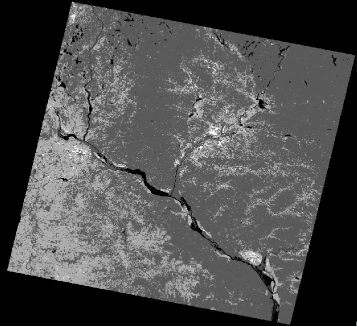
Figure 13: Blackbody radiance temperatures for Landsat 8 thermal image band.

Conclusion

Upon completion of this lab, three different thermal images from three different satellites captured different results for blackbody radiance temperatures. Due to the time differences between the images, the radiance temperatures of various surface features are unique to each image output. To distinguish these differences, the resulting images were brought into ArcMap and the identify tool was used to determine the radiant temperatures of central Lake Wissota in each image. The temperature difference of Lake Wissota between 2000 and 2011 was 262.8°K, or 13.4°F.

Overall, this lab proved how important metadata is to thermal remote sensing, how effective and easy model builder is to use for converting image values from bits to blackbody radiance temperatures, and how temporal resolution affects temperatures of remotely sensed thermal images.

Sources

Data provided by Landsat 8 satellite, U.S. Census Bureau, and Dr. Cyril Wilson
Processing and cartography completed in ERDAS Imagine and ArcMap educational software packages