Lab 3: Unsupervised Classification

Introduction

The goal of this lab was to practice classifying multispectral imagery using unsupervised classification methods in ERDAS Imagine. By learning the input configuration, requirements, execution of unsupervised classification models and recoding spectral clusters of pixel values generated from these models, applications for performing classification in this way is useful for obtaining land use and land cover information.

Methods

Part I: Using Unsupervised ISODATA Classification Algorithm

In the first part of this lab, a multispectral image of the greater Eau Claire area served as the input for an unsupervised classification algorithm using the ISODATA method.

Figure 1: Unsupervised ISODATA classification algorithm model.

In Figure 1, the output image was given a name and storage location, the Method was set to ISODATA, the # of classes was set to 10, and the Maximum Iterations was set to 250. The Approximate True Color option was also selected within the Color Scheme Options window. An output was generated that had a very similar appearance to the input image, with the exception that the resulting image contained 10 discrete color classifications (see Figure 2).

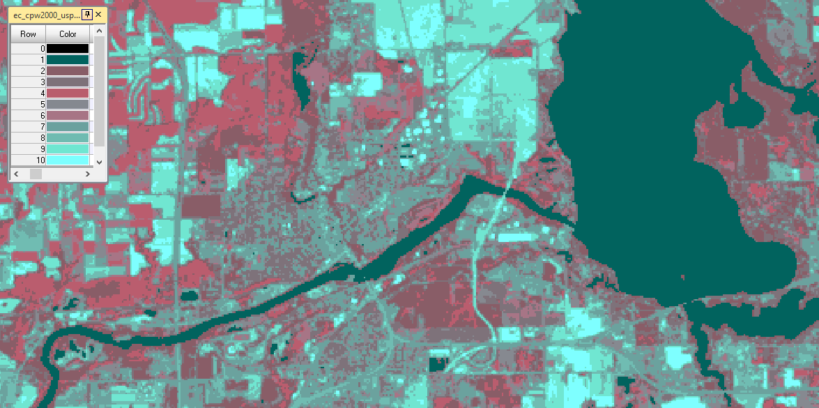Figure 2: Resulting discrete classification image.

In Figure 2, the attribute table for the discrete color classes is shown on the left side of the image, and the discretion of color variance is visible in the image.

Next, this resulting image was given a classification scheme and various classes were labeled to represent true land cover instead of arbitrary colors and numbers. This was done by comparing the multispectral image to a true color satellite image taken near the same time to determine which classes represented which categories of surface feature types. These categories included: water, forest, agriculture, urban/built-up, and bare soil.

Figure 3: Connect and sync to Google Earth viewer.

Using the Link GE to View and Sync GE to View tools shown in Figure 3, the multispectral image displayed in ERDAS Imagine was synced to the same area in Google Earth to compare the spectral classes to their respective surface features in reality.

Figure 4: Changing color of discrete classes.

Once enough surface features were identified for each class, the color representation and label was applied to each class. The 10 classes were reclassified to represent a water, forest, agriculture, urban/built-up, and bare soil lands (see Figure 5).

Figure 5: Resulting classified colors.

Part II: Improving Accuracy of Unsupervised Classification

In the second part of this lab, the goal was to perform similar procedures as in the first part, but increase the accuracy of the classes. This was done by doubling the number of cluster classes produced from the unsupervised classification tool-- which helped reduce the amount of incorrectly classified areas which would be the case when fewer classes are produced.

Figure 6: Unsupervised classification with 20 classes.

In Figure 6, the output image was given a name and storage location, and the rest of the processing options were set to the same values as in the first part with the exception of generating 20 classes instead of 10 (see Figure 7).

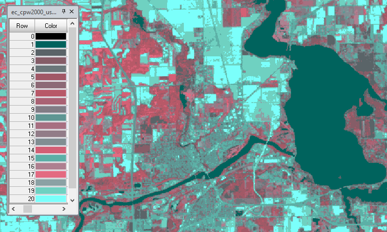Figure 7: Resulting 20-class image.

The classes were recolored and organized in the same way as in part 1-- differentiating between water, forest, agriculture, urban/built-up, and bare soil areas (see Figure 8). Once this was done, the coded values of the classes were changed to match the colored values of the classes previously assigned (see Figure 9).

Figure 8: Resulting classified colors.

Figure 9: Recoding classes.

In Figure 9, the input image was the resulting classified image (shown in Figure 8) and the output image (right side of above image) was given a name and storage location. The coded values for each of the 20 classes was changed to represent their respective classification.

Unclassified = 0
Water = 1
Forest = 2
Agriculture = 3
Urban/Built-up Land = 4
Bare Soil = 5

Once the coded values were reassigned, the associated class color scheme was reapplied using the attribute table.

Figure 10: Resetting color scheme.

Then, a Class Name column was added to the attribute table using the Raster Attribute Editor window, and the class names were entered.

Figure 11: Final unsupervised classification attribute table in ERDAS Imagine.

Then, the classified image was brought into ArcMap to generate the final resulting map showing classified land use and land cover (see Results section).

Results

Figure 12: Resulting land use / land cover map.

Conclusion

The difference between the accuracy of generating 10 classes and 20 classes with an unsupervised classification is slight, but can certainly change from analyst to analyst as well. With unsupervised classification, the algorithms used generate classes based on distinguishable areal units with minimized user error potential, but the analyst does not have much control on how the classes are generated based on what types of land use and land covers are being studied. Since the classification algorithm used in this lab created classes based solely on reflectance, a lot of surface features were incorrectly classified and the spectrum of classes created was limited. Despite correcting for some low-accuracy classification in the second part of this lab by upping the number of classes generated, a lot of roads were grouped in with agriculture-dominant classes and therefore were incorrectly classified, bare soil-dominated classes picked up metallic roofs and other highly reflective surfaces, and mowed fescues (such as lawns, parks, and golf courses) were grouped into agriculture classes, since there wasn't a classification for grasslands.

Overall, this classification method provided a very generalized depiction of land use and land cover for the study area. If one would need incredibly accurate land use and land cover information and time or money was not issue, an unsupervised classification method might not be their best choice; rather, they would be better off completing a supervised classification in which training samples of the study are recorded to generate more accurate classes.

Sources

Data obtained from the Landsat 7 satellite and Dr. Cyril Wilson
Link to Supervised and Unsupervised Classification definition from GIS Geography
Processing and cartography completed in ArcMap and ERDAS Imagine educational software packages