Lab 9: Hyperspectral Remote Sensing

Introduction

The purpose of this lab was to become familiar with various functions and purposes of using hyperspectral data in remote sensing. To perform basic analyses, animation, atmospheric correction, vegetation indices/analyses, and noise transformations, the ENVI image processing software was used.

Methods

Part I: Introduction to Spectral Processing

For the first part of this lab, the objective was to become familiar with basic analyses that can be performed on hyperspectral images using ENVI image processing software.

First, a basic analysis was performed on an image to extract spectral information using the ROI Tool in ENVI. To do this, an image file was brought into a display in ENVI. The image file contained region of interest (ROI) polygons that were then overlayed on the image-- these served as the samples for the ROI Tool to extract the spectral information from the image. Then, the ROI statistics were viewed to determine variances in the spectral profiles of the ROI samples.

Figure 1: ROI tool, statistics, and image with ROIs overlayed.

Next, the spectral signatures of the samples were compared to those of average samples of various minerals: alunite, buddingtonite feldspar, calcite, and kaolinite. This was done by loading the spectral signatures of those minerals into the ROI stats results window.

Figure 2: ROI statistics with mineral spectral profiles.

Part II: Atmospheric Correction Using FLAASH

In the second part of this lab, the objective was to understand how to correct for atmospheric attenuation and produce a reflectance image using the FLAASH method in ENVI.

First, a true color image was brought into an ENVI viewer. The pixel locator viewer function was used to visualize the spectral profile of an urban sample point before atmospheric correction.

Figure 3: Using pixel locator and z profile functions in ENVI image viewer.

The next step was to correct this image using FLAASH. To do this the FLAASH tool was opened from the spectral tab in the main banner. The image shown in the viewer in Figure 3 was used as the input image file, the output file was given a name and storage location, and the "Restore" button was clicked to input a text file which contained ancillary information about the image and sensor it was captured by.

Figure 4: FLAASH input parameters.

Then, the model was applied, it ran, and generated an image and subsequent spectral profile outputs (see Results section).

Part III: Vegetation Analysis

In the third part of this lab, the objective was to explore various vegetation analyses that can be performed on hyperspectral images in ENVI. The first vegetation analysis that was observed was the Vegetation Index Calculator.

To start, a reflective image of the same study area as the image in part 2 was brought into a viewer, ensuring that the red, green, and blue color guns were set to bands 53, 29, and 19 respectively. Then, the spectral tool Vegetation Index Calculator was opened, setting the image in the viewer as the input. The tool parameters window opened (Figure 5) and all vegetation indices were selected, the biophysical cross checking parameter was set to "On", and the output file was given a name and storage location.

Figure 5: Vegetation Index Calculator tool parameters window.

The various vegetation analysis images were brought into viewers and compared. The vegetation indices observed included: normalized difference vegetation index (NDVI), normalized difference lignin index, red edge position index, plant senescence reflectance index, water band index, normalized difference infrared index, and normalized difference water index (NDWI).

Secondly, a few vegetation analysis tools were observed including: agricultural stress tool, fire fuel tool, and forest health tool. The agricultural stress tool assesses the greenness, canopy water content, canopy nitrogen, light use efficiency, and leaf pigment to determine what level of stress the vegetation is undergoing.

Figure 6: Agricultural stress tool parameters.

The output image for this tool can be viewed in the Results section.

The next vegetation analysis tool observed was the fire fuel tool. This tool analyzes an area of vegetation's greenness, canopy water content, and dry or senescent (non-photosynthesizing plants) to determine its flammability.

Figure 7: Fire fuel tool parameters.

The output image for this tool can be viewed in the Results section.

The last vegetation analysis tool used was the forest health tool. Much like determining the stress of agricultural plots, the forest health tool can assess the health of forested vegetation by analyzing the greenness, leaf pigment, canopy water content, and light use efficiency of an area.

Figure 8: Forest health tool parameters.

The output image for this tool can be viewed in the Results section.

Part IV: Hyperspectral Transformation

In the fourth and final part of this lab, the objective was to introduce a method for determining the inherent dimensionality of image data, segregate noise in the data, and reduce computational requirements for processing hyperspectral images. This method is called the Minimum Noise Fraction Transformation (MNF).

Figure 9: MNF process flow.

To do this, an image was brought into an ENVI viewer and the Estimate Noise Statistics tool was used from the "Transform" tab in the main banner. The image was then subset to a part of the image with a good amount of noise. Finally, the statistics were calculated.

Figure 10: Inputting image into Estimate Noise Statistics tool.

Figure 11: Subsetting the imagery.

The resulting Eigen values can be viewed in the Results section.

Results

Figure 12: Output for FLAASH correction.

In Figure 12, the image and subsequent spectral profile on the left represents the uncorrected image and on the right is the FLAASH corrected image. Parts of the corrected spectral profile are missing due to the tool removing problematic bands that were causing the image to appear hazy and not true to ground color.

Figure 13: Agricultural Stress tool output.

In Figure 13, purple represents areas of vegetation with the least amount of stress and areas of red represent areas with the most amount of stress. The areas in the above image that are experiencing the most stress are the roads. This is an obvious result as they are not green, have little to no water content, do not store or use nitrogen from the soil, and are highly reflective of visible light-- all of which would be characteristics of very unhealthy vegetation if these areas were vegetation. An urban mask was used in the following outputs to avoid this.

Figure 14: Fire Fuel tool output.

In a similar way as Figure 13, Figure 14 shows blue areas as being least likely to catch fire and red areas as being most likely to catch fire. In this image, an urban mask was used to not include urban areas (roads, buildings, other inorganic human-made structures) so that only vegetation was being assessed.

Figure 15: Forest Health tool output.

In Figure 15, blue represents areas of low forest health and red represents areas of high forest health. Again, the urban mask was used to deter non-forested areas from being included in the algorithm.

Figure 16: MNF z profile output.

In Figure 16, the output from the hyperspectral transformation is shown.

Conclusion

As shown in this lab, there are many uses for hyperspectral imagery in various spectral analysis. Whether it's determining differences in mineral types, correcting effects of atmospheric attenuation, assessing various health characteristics of vegetation, or circumventing noise contained within an image, hyperspectral remote sensing can aid analyses that would not be possible with multispectral images alone.

Sources

Dr. Cyril Wilson

Support. (n.d.). Retrieved from http://www.harrisgeospatial.com/Support/SelfHelpTools/Tutorials.aspx

Lab 8: Advanced Image Classifiers

Introduction

The goal of this lab was to build on knowledge of classification methods obtained from previous labs by examining advanced classification schemes. Differing from un/supervised classification methods, advanced classifiers use complex decision trees and neural networks to learn from user input and build a classification scheme in an image.

Methods

Part I: Expert System Classification

The first advanced classifier used in this lab was an "expert system". An expert system uses the spectral information from the image to generate a classification scheme, much like un/supervised algorithms, but also as much ancillary data as is available. So information regarding temperature, soil, zoning, population, and a plethora of other information that supplements assessment of the surface features in the image is used to generate a better than minimum threshold classified image.

To begin the expert system classification process, a classified image was brought into ERDAS Imagine and observed. This was done by comparing the classified image to a Google Earth image of the same area. The greatest misclassified fields were lawns and other open grass areas that were classified as agriculture- this was corrected using the expert classification scheme. Through this process, the "urban/built-up" class was split into "residential" and "other urban" as well.

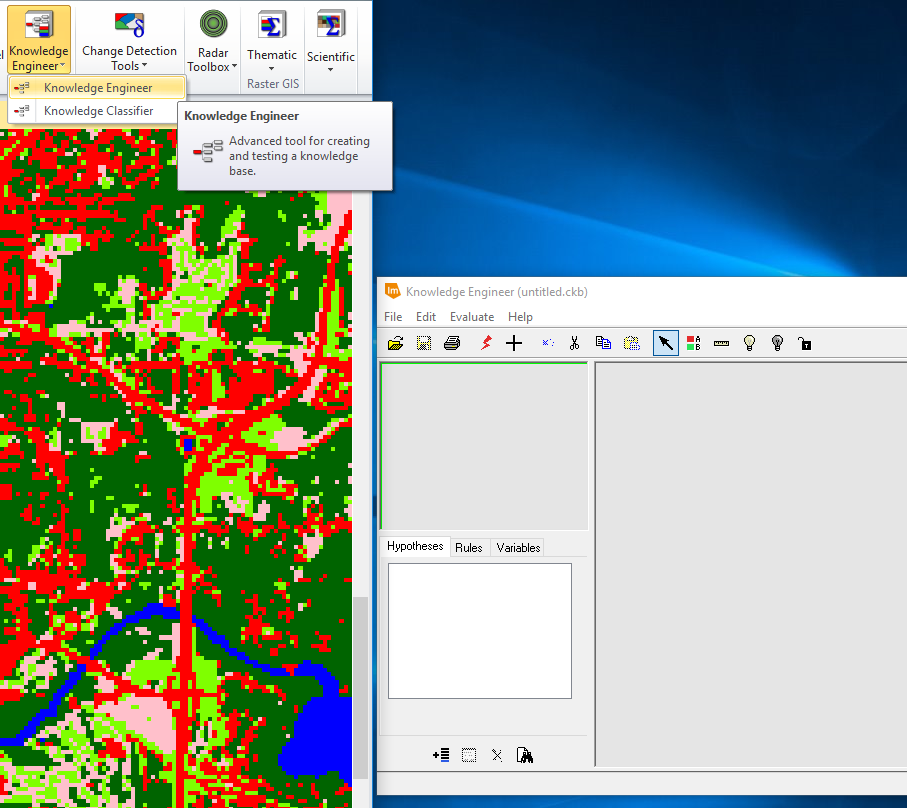
Once the classes needing correction were identified, the Knowledge Engineer raster tool was used to train the classifier.

Figure 1: Opening the Knowledge Engineer raster tool.

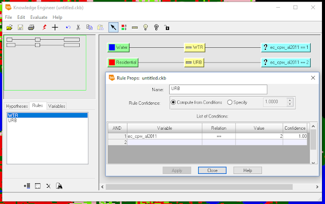
Figure 2: Setting rules for class values within the Knowledge Engineer.

By creating a "Hypothesis Class" (two of which are shown as the green tabs in Figure 2) for each class in the image and setting the "Rule Props" (shown in "rule props" window in Figure 2) to associate a value with each class in the image, the Knowledge Engineer established rules for the expert classifier to follow.

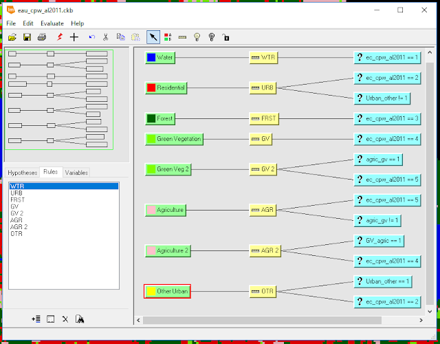
Figure 3: Finalized Knowledge Engineer trainer.

As shown in Figure 3, every class that was included in the original classified image was included here, but also a few other classes were added ("Green Veg 2", "Agriculture 2", and "Other Urban" hypothesis classes). Also, notice that there are a few classes with two values-- this was a result of a logical operation created in the rules which is what trains the reclassification scheme to choose whether a class is as classified or should be changed using ancillary data (shown as variables in Figure 3 that do not use the image in question "ec_cpw_al2011").

Once the Knowledge Engineer was finished, the engineer was ran to verify that the trainer was set up properly. The engineer was then used to train the Knowledge Classifier raster tool.

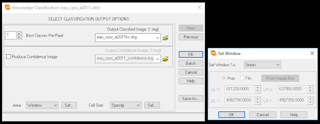
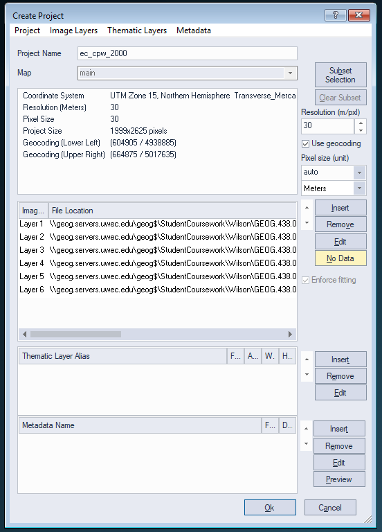
Figure 4: Inputting parameters to the Knowledge Classifier.

In Figure 4, the output image was given a name and storage location, the "Area" parameter was set to "Union" (shown in the "Set Window" window), and the "Cell Size" parameter was set to 30 x 30. The output image was generated (see Results section).

Part II: Neural Network Classification

The second part of this lab focused on a different kind of advanced classifier-- the Neural Network classifier. This classification method simulates a network of neural pathways in the human brain. To do this, ENVI software was used. First, an image was brought into the software and the color bands of that image were selected to bring the image into a viewer.

Figure 5: Selecting color band combination to display a false color image.

Once the color band combination was determined, the next step was to restore the predefined regions of interest (ROIs) within the image; these were displayed as red, green, and blue polygons that overlayed the image.

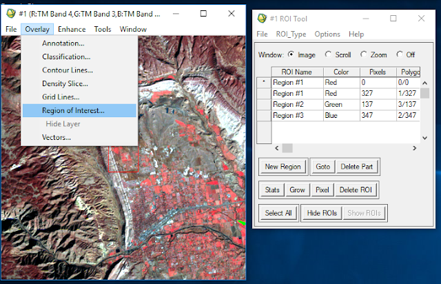
Figure 6: Restoring ROIs.

Then, the neural network parameters were established

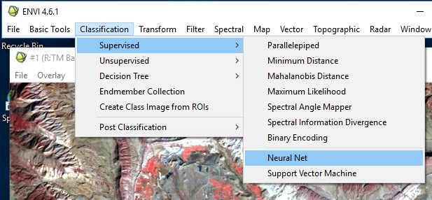
Figure 7: Starting neural network classification.

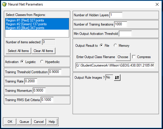
Figure 8: Establishing parameters for neural network.

In Figure 8, the red, green, and blue regions were selected as classes (these were based on the polygons overlayed in the original image), the activation parameter was set to "logistic", the number of training iterations was set to 1000, the output file was given a name and storage location, and the output rule images parameter was set to "no". This model was then ran and produced an RMS error by number of iterations plot and a classified version of the input image (see Results section).

Results

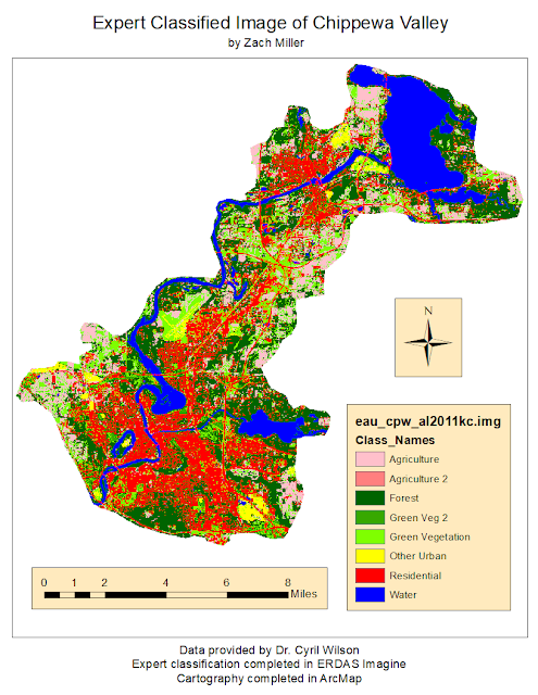
Figure 10: Expert classification result.

Looking at the results of part one (Figure 10), the image displays a more accurate and detailed classification than the input classified image (Figure 9). The output from the expert system splits the urban/built-up land into residential and other urban, which is distinguishable in many areas within the image-- the Chippewa Valley Regional Airport on mid-west side and Maple Wood Mall on southeast side of the image are good examples of this change. One issue with the expert system output, however, is that the resulting agriculture and green vegetation classes are unintentionally split into two classes which makes the output more confusing in my opinion. On the other hand, this could be useful in determining which areas were changed to agriculture and green vegetation as a result of using the expert system.

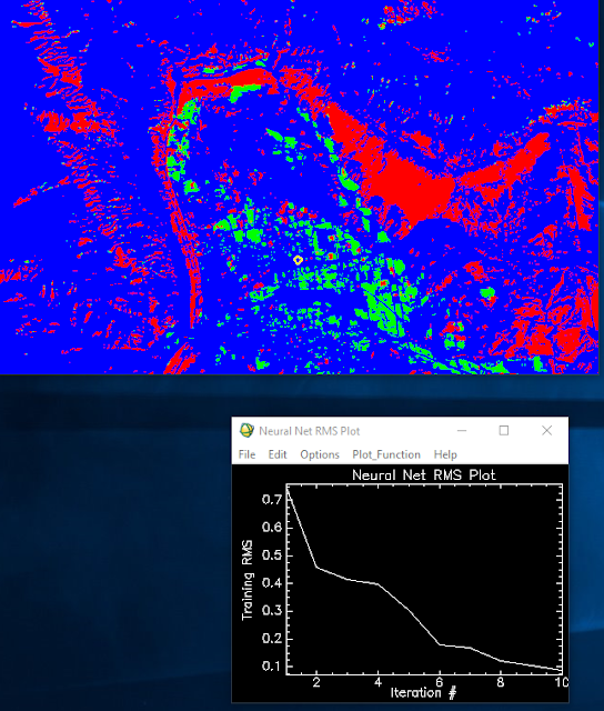
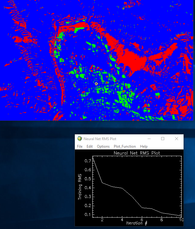
Figure 11: Neural Network output image and RMS plot.

Looking at the results shown in Figure 11, the image was split into 3 distinct classes based on the sample polygons overlayed on the multispectral image. The neural network appeared to have only required ten iterations to achieve a less than 0.1 root mean square (RMS) error as well-- which seems quick to my relatively inexperienced understanding of the neural network function in ENVI. 

Conclusion

The expert system classification has proven to expertly distinguish differences and therefore, enhance classified imagery. Despite the inability to combine classes that were split in the knowledge engineer (ie. green vegetation [1 and 2] and agriculture[1 and 2]), which was most likely user error, the method adequately supplements the original classification to create a more accurate output and give the viewer a better understanding of the LULC within the study area.

As for the neural network, the objectives and output seem less clear. The resulting classes seem meaningless or at least indistinguishable as to what they are supposed to represent. The overall process and software was confusing to operate and derive meaningful results from. Having worked through the lab and read the support documents for what the system and function do, I still don't have a good grasp on how either work or what the point of using them is.

Overall, I was quite pleased, and frankly surprised, at the output generated from the expert system classification and could envision using that method for future projects having to do with classification. I would be interested to learn more about the functionality and various uses for employing a neural network classifier, as I felt that the scenario for this assignment didn't provide enough information to allow me to fully grasp the concepts of this classification method.

Sources

Department of Geography, University of Northern Iowa [Quickbird Highresolution Image]. (n.d.).

Earth Resource Observation and Science Center [Landsat Satellite Images]. (n.d.).

United States Geological Survey [Landsat Satellite Images]. (n.d.).

ment of Geography, University of Northern Iowa [Quickbird Highresolution Image]. (n.d.).

Earth Resource Observation and Science Center [Landsat Satellite Images]. (n.d.).

United States Geological Survey

Department of Geography, University of Northern Iowa [Quickbird Highresolution Image]. (n.d.).

Earth Resource Observation and Science Center [Landsat Satellite Images]. (n.d.).

United States Geological Survey [Landsat Satellite Images]. (n.d.).

Department of Geography, University of Northern Iowa [Quickbird Highresolution Image]. (n.d.).

Earth Resource Observation and Science Center [Landsat Satellite Images]. (n.d.).

United States Geological Survey [Landsat Satellite Images]. (n.d.).

Department of Geography, University of Northern Iowa [Quickbird Highresolution Image]. (n.d.).

Earth Resource Observation and Science Center [Landsat Satellite Images]. (n.d.).

United States Geological Survey [Landsat Satellite Images]. (n.d.).

Department of Geography, University of Northern Iowa [Quickbird Highresolution Image]. (n.d.).

Earth Resource Observation and Science Center [Landsat Satellite Images]. (n.d.).

United States Geological Survey [Landsat Satellite Images]. (n.d.).

Lab 7: Object-based Classification

Introduction
Methods
Part I: Create a New Project in eCognition Developer

In the first part of this lab, the goal was to, as the name implies, create a new project in eCognition Developer. The first step after opening the software was to bring in an image of the greater Eau Claire area and change the spectral band combination to reflect a false color image instead of the default color combination.

Figure 1: Creating a new project and importing the image.

Figure 2: Changing the spectral band combination to reflect a false color image.

Part II: Segmentation and Sample Collection

Next, the Process Tree function in eCognition was used to generate polygons that segmented the image. This was done by appending a new process to the window (Lab7_object_classification in Figure 4), inserting a child process (generate objects in Figure 4), and inserting another child process (Level 1 in Figure 4). The polygons for 'Level 1' were generated (Figure 5) after the settings for the process were established (Figure 4).

Figure 3: Opening a Process Tree Dialogue Window.

Figure 4: Branches of process tree shown in upper right, settings for 'Level 1' process shown in Edit Process window.

The multiresolution segmentation process was executed to segment the image (Figure 5).

Figure 5: Segmented image.

Once, the image was segmented, the next step was to generate a classification scheme and select training samples based on that classification scheme.

Figure 6: Classification hierarchy/scheme.

Figure 7: Selecting training samples, the objects that are being used to train the classifier are highlighted in the color they represent in the classification scheme.

A sufficient amount of training samples with varying spectral signatures was necessary to properly train the classifier, the following guideline was used:

Table 1: Minimum amount of required training samples for each class.

Part III: Implementing Object Classification

Once the training samples were collected, they needed to be put to use. The first step in this process was to create the classifier variable. This was done by selecting Process>Manage Variable in the banner of eCognition. A new variable was added, given a name of "RF Classifier" and "string" data type. The variable was then created and the Manage Variables window was exited.

Figure 8: Create new scene variable.

Next, a few more processes were added to the process tree which sought to train and apply the classifier based on the samples collected in the last part of this lab. First, a new process was appended to the process tree, just below the segmentation process. This was given a name of "RF Classification"-- a similar name to the variable created in Figure 8. A child was inserted below this process and given a name of "Train RF Classifier", and another child was inserted within the previous process (Figure 9).

Figure 9: Train Classifier process.

The process shown in Figure 9 is what gives functionality to the trainer. The features that were selected included:

Figure 10: Select features.

Then, another child was inserted into the RF Classification process to apply the RF Classification after the classifier was trained.

Figure 11: Train classifier to apply RF Classification.

With all processes for object-based classification done, the process tree was executed to classify the image. See Results for initial classified image. Of course, the initial classification was not perfect and required some