Lab 9: Hyperspectral Remote Sensing

Introduction

The purpose of this lab was to become familiar with various functions and purposes of using hyperspectral data in remote sensing. To perform basic analyses, animation, atmospheric correction, vegetation indices/analyses, and noise transformations, the ENVI image processing software was used.

Methods

Part I: Introduction to Spectral Processing

For the first part of this lab, the objective was to become familiar with basic analyses that can be performed on hyperspectral images using ENVI image processing software.

First, a basic analysis was performed on an image to extract spectral information using the ROI Tool in ENVI. To do this, an image file was brought into a display in ENVI. The image file contained region of interest (ROI) polygons that were then overlayed on the image-- these served as the samples for the ROI Tool to extract the spectral information from the image. Then, the ROI statistics were viewed to determine variances in the spectral profiles of the ROI samples.

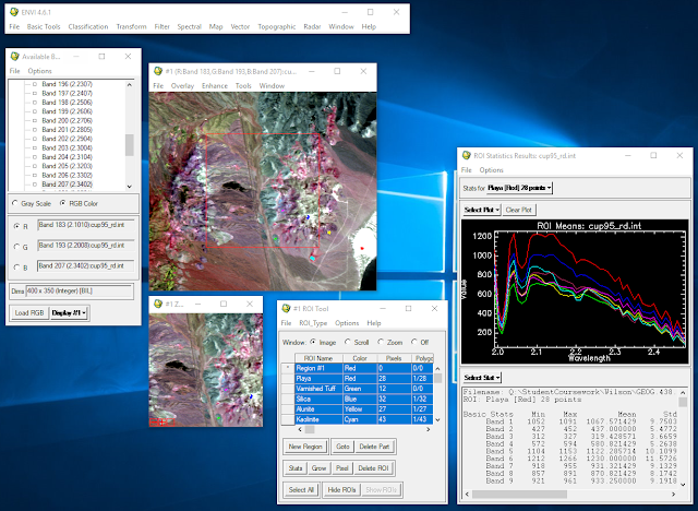Figure 1: ROI tool, statistics, and image with ROIs overlayed.

Next, the spectral signatures of the samples were compared to those of average samples of various minerals: alunite, buddingtonite feldspar, calcite, and kaolinite. This was done by loading the spectral signatures of those minerals into the ROI stats results window.

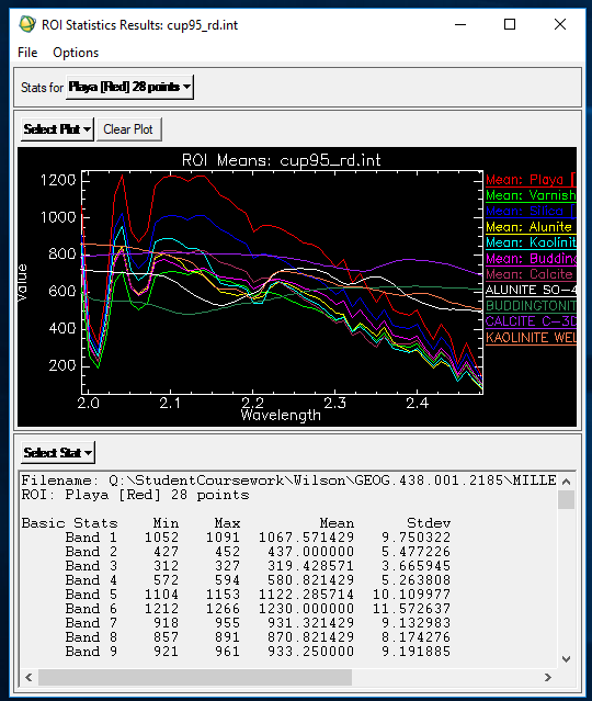Figure 2: ROI statistics with mineral spectral profiles.

Part II: Atmospheric Correction Using FLAASH

In the second part of this lab, the objective was to understand how to correct for atmospheric attenuation and produce a reflectance image using the FLAASH method in ENVI.

First, a true color image was brought into an ENVI viewer. The pixel locator viewer function was used to visualize the spectral profile of an urban sample point before atmospheric correction.

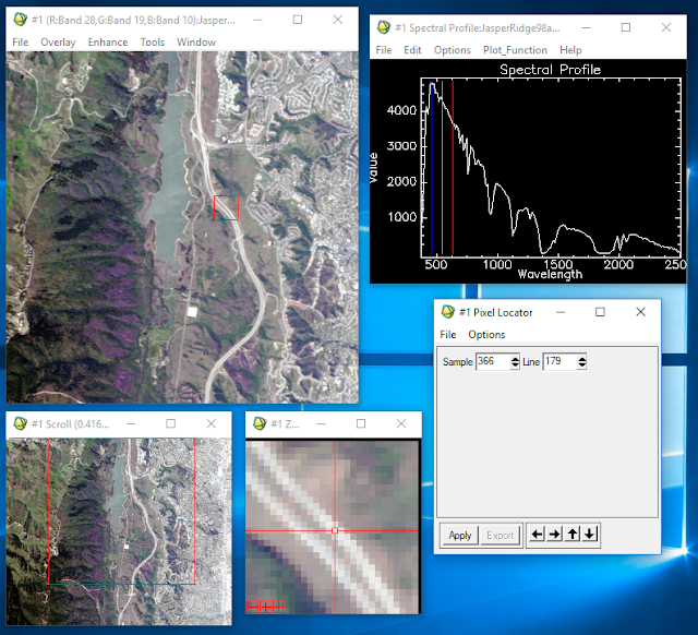Figure 3: Using pixel locator and z profile functions in ENVI image viewer.

The next step was to correct this image using FLAASH. To do this the FLAASH tool was opened from the spectral tab in the main banner. The image shown in the viewer in Figure 3 was used as the input image file, the output file was given a name and storage location, and the "Restore" button was clicked to input a text file which contained ancillary information about the image and sensor it was captured by.

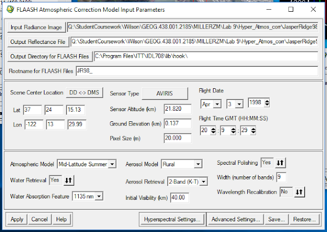Figure 4: FLAASH input parameters.

Then, the model was applied, it ran, and generated an image and subsequent spectral profile outputs (see Results section).

Part III: Vegetation Analysis

In the third part of this lab, the objective was to explore various vegetation analyses that can be performed on hyperspectral images in ENVI. The first vegetation analysis that was observed was the Vegetation Index Calculator.

To start, a reflective image of the same study area as the image in part 2 was brought into a viewer, ensuring that the red, green, and blue color guns were set to bands 53, 29, and 19 respectively. Then, the spectral tool Vegetation Index Calculator was opened, setting the image in the viewer as the input. The tool parameters window opened (Figure 5) and all vegetation indices were selected, the biophysical cross checking parameter was set to "On", and the output file was given a name and storage location.

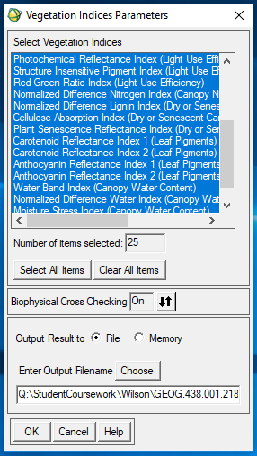Figure 5: Vegetation Index Calculator tool parameters window.

The various vegetation analysis images were brought into viewers and compared. The vegetation indices observed included: normalized difference vegetation index (NDVI), normalized difference lignin index, red edge position index, plant senescence reflectance index, water band index, normalized difference infrared index, and normalized difference water index (NDWI).

Secondly, a few vegetation analysis tools were observed including: agricultural stress tool, fire fuel tool, and forest health tool. The agricultural stress tool assesses the greenness, canopy water content, canopy nitrogen, light use efficiency, and leaf pigment to determine what level of stress the vegetation is undergoing.

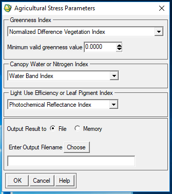Figure 6: Agricultural stress tool parameters.

The output image for this tool can be viewed in the Results section.

The next vegetation analysis tool observed was the fire fuel tool. This tool analyzes an area of vegetation's greenness, canopy water content, and dry or senescent (non-photosynthesizing plants) to determine its flammability.

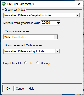Figure 7: Fire fuel tool parameters.

The output image for this tool can be viewed in the Results section.

The last vegetation analysis tool used was the forest health tool. Much like determining the stress of agricultural plots, the forest health tool can assess the health of forested vegetation by analyzing the greenness, leaf pigment, canopy water content, and light use efficiency of an area.

Figure 8: Forest health tool parameters.

The output image for this tool can be viewed in the Results section.

Part IV: Hyperspectral Transformation

In the fourth and final part of this lab, the objective was to introduce a method for determining the inherent dimensionality of image data, segregate noise in the data, and reduce computational requirements for processing hyperspectral images. This method is called the Minimum Noise Fraction Transformation (MNF).

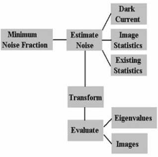Figure 9: MNF process flow.

To do this, an image was brought into an ENVI viewer and the Estimate Noise Statistics tool was used from the "Transform" tab in the main banner. The image was then subset to a part of the image with a good amount of noise. Finally, the statistics were calculated.

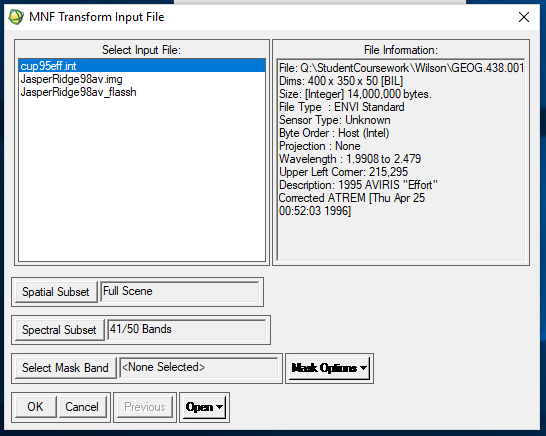Figure 10: Inputting image into Estimate Noise Statistics tool.

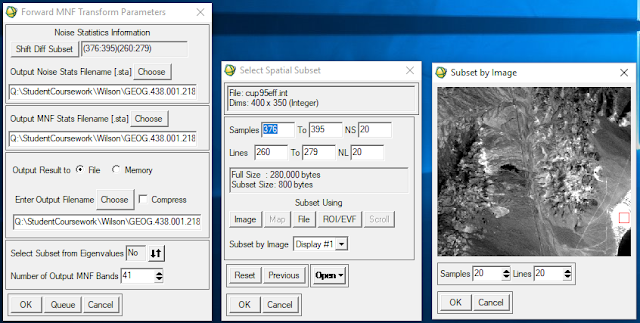Figure 11: Subsetting the imagery.

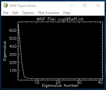
The resulting Eigen values can be viewed in the Results section.

Results

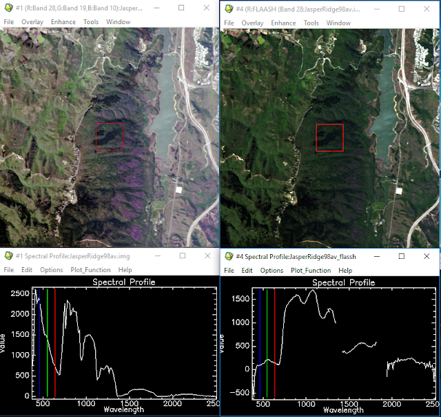Figure 12: Output for FLAASH correction.

In Figure 12, the image and subsequent spectral profile on the left represents the uncorrected image and on the right is the FLAASH corrected image. Parts of the corrected spectral profile are missing due to the tool removing problematic bands that were causing the image to appear hazy and not true to ground color.

Figure 13: Agricultural Stress tool output.

In Figure 13, purple represents areas of vegetation with the least amount of stress and areas of red represent areas with the most amount of stress. The areas in the above image that are experiencing the most stress are the roads. This is an obvious result as they are not green, have little to no water content, do not store or use nitrogen from the soil, and are highly reflective of visible light-- all of which would be characteristics of very unhealthy vegetation if these areas were vegetation. An urban mask was used in the following outputs to avoid this.

Figure 14: Fire Fuel tool output.

In a similar way as Figure 13, Figure 14 shows blue areas as being least likely to catch fire and red areas as being most likely to catch fire. In this image, an urban mask was used to not include urban areas (roads, buildings, other inorganic human-made structures) so that only vegetation was being assessed.

Figure 15: Forest Health tool output.

In Figure 15, blue represents areas of low forest health and red represents areas of high forest health. Again, the urban mask was used to deter non-forested areas from being included in the algorithm.

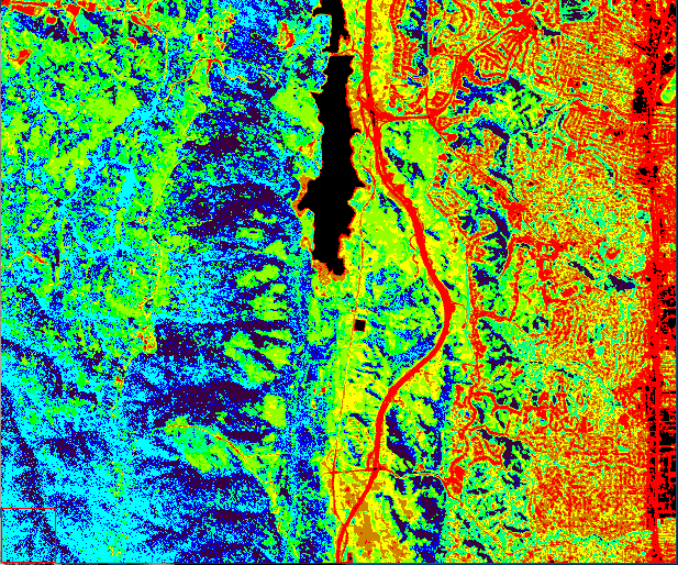
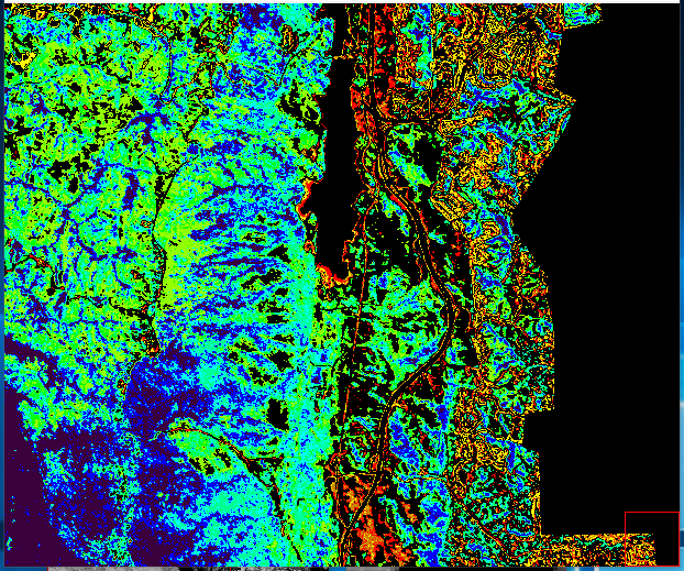
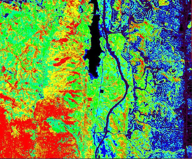
Figure 16: MNF z profile output.

In Figure 16, the output from the hyperspectral transformation is shown.

Conclusion

As shown in this lab, there are many uses for hyperspectral imagery in various spectral analysis. Whether it's determining differences in mineral types, correcting effects of atmospheric attenuation, assessing various health characteristics of vegetation, or circumventing noise contained within an image, hyperspectral remote sensing can aid analyses that would not be possible with multispectral images alone.

Sources

Dr. Cyril Wilson

Support. (n.d.). Retrieved from http://www.harrisgeospatial.com/Support/SelfHelpTools/Tutorials.aspx