Lab 6: Digital Change Detection

Introduction

The goal of this lab was to examine different procedures of detecting land use / land cover (LULC) change over time with satellite images. The procedures and methods used in this lab allowed qualitative, quantitative, and LULC from-to information.

Methods

Part I: Change Detection using Write Function Memory Insertion

In the first part of this lab, the goal was to visualize changes in LULC by assessing significant differences in the near infrared bands of two satellite images taken 20 years apart. To do this, a layer stack was performed on the two images using the Raster>Spectral tool set in ERDAS Imagine. The output image was given a name and storage location.

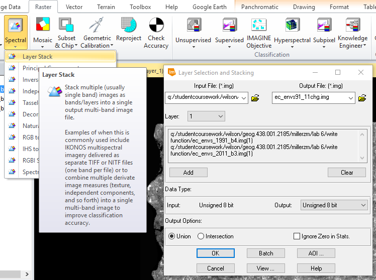
Figure 1: Performing a layer stack on the 1991 and 2011 images.

Once the NIR layers were stacked together, the Multispectral>Bands tool set was used to display the NIR bands from each image in the red, green, and blue bands which displayed the areas that changed in red and the areas that didn't change in blue.

Figure 2: Setting layer combinations.

Part II: Post-Classification Comparison Change Dectection

Section I:

In the second part of this lab, the goal was to practice deriving quantitative data from change detection. To do this, the class and histogram values of two classified images covering the Milwaukee Metropolitan Statistical Area (MSA) were put into an excel sheet to calculate the percentage of change within each class.

Figure 3: Class coverage in hectares (Ha) and the percent of change between within each class between 2001 and 2011.

The hectare values for each image were calculated based on the histogram values for each band, the spatial resolution of the images, and the meters to hectares conversion.

Section II:

Although in the last section, the percent of change for each classification was determined, information regarding what classes changed from-to was not. In this section of the lab, the two images of the greater Milwaukee MSA from 2001 and 2011 were brought into model builder to determine class changes between the two image dates. The from-to changes were:

1. Agriculture to Urban/Built up
2. Wetlands to Urban/Built up
3. Forest to Urban/Built up
4. Wetland to Agriculture
5. Agriculture to Bare Soil

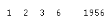
Figure 4: Class Values used for model builder function.

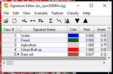
Figure 5: Testing for wetland areas in 2001 image.

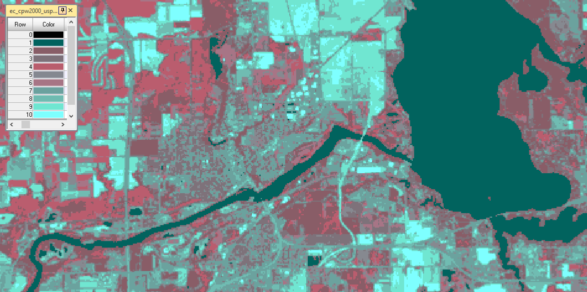
Figure 6: Testing for Urban/Built up areas in 2011 image.

By using the two images as inputs for 10 functions within model builder, the images were tested for the various from-to classes in question using a conditional statement. In figures 5 and 6. The 2001 and 2011 images were being tested for wetland and urban/built-up land. All wetland areas within the 2001 image were assigned a value of 1 and all others, 0. All Urban/Built-up land in the 2011 image was assigned a value of 1 and all others, 0. This produced a binary image for both years, which were then used to determine which land changed between the two dates.

Figure 7: Bitwise function used to compare the two images.

The images were then brought into ArcMap to visualize the from-to changes.

Results

Figure 8: Agriculture to Urban/Built-up Change Detection Map.

Figure 9: Wetland to Urban/Built-up Change Detection Map.

Figure 10: Forest to Urban/Built-up Change Detection Map.

Figure 11: Wetland to Agriculture Change Detection Map.

Figure 12: Agriculture to Bare Soil Change Detection Map.

The various mapped results display different amounts of from-to changes. The change between 2001 and 2011 from Agriculture to Urban/Built-up land (Figure 8) is quite extensive as compared to the change from Agriculture to Bare Soil (Figure 12).

Conclusion

Looking at the methods used in Part 1 of this lab, the Write Memory Function does a good job of highlighting whether or not change occurred in the area of study over two dates, but did not provide quantitative information regarding what changed and what from-to. 

Looking at the results from Part II, the Post-Classification Comparison Change Detection method provided information about what changes occurred between the two image dates and was relatively easy to perform using the Wilson-Lula method in Model Builder. This process also provided quantitative information regarding percent change, which was not given by the Write Memory Function.

Sources

Classified images provided by Dr. Cyril Wilson

Processing executed in ERDAS Imagine

Cartography completed in ArcMap 10.5.1

Lab 5: Classification Accuracy Assessment

Introduction

Methods

Part I: Generating Ground Reference Testing Samples for Accuracy Assessment

In the first part of this lab, the classified image created in Lab 3 was used in conjunction with a high-resolution image of the same area from the National Agriculture Imagery Program (NAIP) to assess the accuracy of the classified image. First, sample testing points were generated. This was completed by using the Accuracy Assessment raster tool in ERDAS Imagine.

Figure 1: Adding random sample points to the reference image (high-resolution image on right).

 In Figure 1, the Create/add random points command was selected to open the Add Random Points window and the classes from the classified image (on left) were selected in the Raster Attribute Editor window. The points were generated in the Accuracy Assessment window and displayed in the reference image window.

Figure 2: Randomly generated points.

Part II: Performing Accuracy Assessment

The points were then classified, 10 at a time, using the same classification scheme from Lab 3 and the reference image to determine the true land use/cover. Once this was done, an accuracy report was generated using the Report > Accuracy Report and interpreted to determine the overall accuracy of the classified imagery.

Figure 3: Accuracy Report Totals.

Values from the accuracy report were put into an Error Matrix which visualizes the erroneous classes.

Figure 4: Error Matrix for the unsupervised classified image. Classes displayed along Y-axis and the reference image is displayed along the X-axis. 

The Error Matrix shown in Figure 4, displays which land use / land covers (left-most column) were classified as the land use / land covers along the top-most row. For example, within the "Urban/Built-up" row, 12 points that were urban in the reference image were classified as agriculture and 6 classified as bare soil in the unsupervised classified image.

Part III: Accuracy Assessment of Supervised Classification

For the third and final part of this lab, the same processes completed in parts one and two were completed for the supervised classified image created in Lab 4. The Accuracy Report was generated,

Figure 5: Accuracy Report Totals.

and the values for each class were entered into an Error Matrix.

Figure 6: Error matrix for the supervised classified image.

Results

Looking at the resulting error matrices and accuracy reports, the unsupervised classified image was more accurate than the supervised classified image. While both the producers and users accuracy in the unsupervised and supervised images were 0%, the forest and agriculture classes were more accurately classified in the unsupervised image than in the supervised image. The bare soil class was more accurately classified in the supervised image than in the unsupervised image, however. In terms of reliability (user's accuracy), the forest and bare soil classes in the supervised image are trustworthy in the supervised image than in the unsupervised image and the agriculture class displayed the opposite.

Conclusion

Overall, the accuracy of any class, with the exception of water, in either classification method was less than impressive. Considering that the urban/built-up class is considered completely unreliable by the accuracy report, although there are some areas that are correctly classified as such in either image, this is an area of much concern. Aside from water, forested lands were the only acceptable class in either image for reliability, as agricultural and bare soil areas fell below 40% confidence in both accuracy reports. Perhaps the random sample point selection method is to blame for disproportionally placing points on forested areas where it would have been helpful to have more points placed on urban areas to better determine the accuracy of that class.

Sources

Reference images collected by the National Agriculture Imagery Program (NAIP)
Accuracy assessment completed in ERDAS Imagine
Error matrices designed in Microsoft Excel
References:
Accuracy Metrics. (n.d.). Retrieved March 14, 2018, from http://gsp.humboldt.edu/olm_2016/Courses/GSP_216_Online/lesson6-2/metrics.html
Reference for "Producer and User Accuracy"

Lab 4: Pixel-Based Supervised Classification

Introduction

The goal of this lab was to become familiar with supervised classification, which differs from unsupervised classification learned last lab. With this method of classification, the user is given more control over the classes generated by the software, which in this case is ERDAS Imagine.

Methods

Part I: Collection of Training Samples for Supervised Classification

In the first part of this lab, the objective was to collect various land use/land cover samples to "train" the classification scheme, as the name of this section implies, through the use of drawing polygons and inputting them as areas of interest (AOIs) in the signature editor window.

Figure 1: Adding a polygon to the signature editor (as an AOI).

In Figure 1, the yellow polygon shown on the left side of the image represents a training sample used for the water classification, and the red box highlighted on the right side of the image represents the Signature Editor window with the lake AOI shown as Class 1. This title was later changed to say "Water 1" and 11 more training samples were collected for water. Forest, agriculture, urban/built-up land, and bare soil samples were also collected through a similar procedure; in total, 50 signatures were used.

Figure 2: Completed signature editor.

In Figure 2, the signature editor window is displayed having 50 sample signatures with different labels to reflect the land cover/land use of each associated polygon. Google Earth was used to verify that the sample signature being collected was accurate.

Part II: Evaluating the Quality of Training Samples

In the second part of this lab, the goal was to evaluate the training samples collected from part 1, by ensuring that their spectral signatures represented those of their respective land uses/land covers in the signature editor window. Then, the samples were compiled to create supervised classes of each of the land uses/land covers.***

Figure 3: Displaying the mean plot of water signatures collected from part 1.

In Figure 3, the Signature Mean Plot window is shown on the right side. This displays the mean reflectance in each spectral band for all water samples collected. The purpose of this step was to identify any outliers. If one spectral signature looked completely different than the majority, that sample was deleted and a new sample was created. This was done with the rest of the class samples.

Next, the separability between the class samples were evaluated by first adding the spectral signatures of all samples collected to one signature editor window, then running an Evaluate Signature Separability model (see Figure 4).

Figure 4: Evaluating signature separability in the signature editor window.

Figure 5: The spectral bands with the greatest separability between classes are on the left (1, 2, 3, and 6), and the average separability score is shown on the right (1956).

After running the model shown in Figure 4, a separability report was generated and the numbers shown in Figure 5, were captured from that report. Based on the sample signatures collected, the spectral bands that display the greatest separability between classes are the blue, green, red, and near infrared (NIR) bands; and this is what the classification scheme should be based on. The average separability score shown in Figure 5, "1956", means that the amount of separability within the class sample signatures was sufficient and classification could commence. The next step was to merge all of the classes into individual discrete classes by using the Merge function in the Signature Editor Window (see Figure 6).

Figure 6: Discrete classes.

The raster tool, Supervised Classification, was then used to classify the rest of the image based on the mean sample signatures (see Figure 7).

Figure 7: Running a supervised classification model.

In Figure 7, the input image was the multispectral image shown in the background, the input signature file was the signature editor created in the previous step (see Figure 6), and the classified file was the output image which was given a name and location.

Once the output image was generated, it was compared to the unsupervised image (see Results).

Results

Figure 8: Completed supervised classification map.

Conclusion

Looking at the results, this classification scheme did not produce an accurate result. Urban/ built-up land dominates the image when in reality, there are a lot of misclassified areas to the far east, west, and south of the Eau Claire and Chippewa Falls areas that are predominantly agriculture and forest. A lot of water was misclassified as urban/ built-up land as well. The section of the Eau Claire river between Lake Altoona and Lake Eau Claire provides a good example of this, but also, there are parts of the Chippewa river just southwest of Eau Claire that was classified as urban/built-up land. The reason for this poor accuracy could have something to do with the variety of spectral signatures for urban/ built-up land. Since roof tops, roads, and other highly reflective surfaces and materials were sampled as urban/built-up classes, some of the spectral signatures of agriculture, water, and bare soil were incorrectly grouped in with the urban/built-up class.

Sources

Landsat 5, Dr. Cyril Wilson, Google Earth, ArcMap, and ERDAS Imagine

Lab 3: Unsupervised Classification

Introduction

The goal of this lab was to practice classifying multispectral imagery using unsupervised classification methods in ERDAS Imagine. By learning the input configuration, requirements, execution of unsupervised classification models and recoding spectral clusters of pixel values generated from these models, applications for performing classification in this way is useful for obtaining land use and land cover information.

Methods

Part I: Using Unsupervised ISODATA Classification Algorithm

In the first part of this lab, a multispectral image of the greater Eau Claire area served as the input for an unsupervised classification algorithm using the ISODATA method.

Figure 1: Unsupervised ISODATA classification algorithm model.

In Figure 1, the output image was given a name and storage location, the Method was set to ISODATA, the # of classes was set to 10, and the Maximum Iterations was set to 250. The Approximate True Color option was also selected within the Color Scheme Options window. An output was generated that had a very similar appearance to the input image, with the exception that the resulting image contained 10 discrete color classifications (see Figure 2).

Figure 2: Resulting discrete classification image.

In Figure 2, the attribute table for the discrete color classes is shown on the left side of the image, and the discretion of color variance is visible in the image.

Next, this resulting image was given a classification scheme and various classes were labeled to represent true land cover instead of arbitrary colors and numbers. This was done by comparing the multispectral image to a true color satellite image taken near the same time to determine which classes represented which categories of surface feature types. These categories included: water, forest, agriculture, urban/built-up, and bare soil.

Figure 3: Connect and sync to Google Earth viewer.

Using the Link GE to View and Sync GE to View tools shown in Figure 3, the multispectral image displayed in ERDAS Imagine was synced to the same area in Google Earth to compare the spectral classes to their respective surface features in reality.

Figure 4: Changing color of discrete classes.

Once enough surface features were identified for each class, the color representation and label was applied to each class. The 10 classes were reclassified to represent a water, forest, agriculture, urban/built-up, and bare soil lands (see Figure 5).

Figure 5: Resulting classified colors.

Part II: Improving Accuracy of Unsupervised Classification

In the second part of this lab, the goal was to perform similar procedures as in the first part, but increase the accuracy of the classes. This was done by doubling the number of cluster classes produced from the unsupervised classification tool-- which helped reduce the amount of incorrectly classified areas which would be the case when fewer classes are produced.

Figure 6: Unsupervised classification with 20 classes.

In Figure 6, the output image was given a name and storage location, and the rest of the processing options were set to the same values as in the first part with the exception of generating 20 classes instead of 10 (see Figure 7).

Figure 7: Resulting 20-class image.

The classes were recolored and organized in the same way as in part 1-- differentiating between water, forest, agriculture, urban/built-up, and bare soil areas (see Figure 8). Once this was done, the coded values of the classes were changed to match the colored values of the classes previously assigned (see Figure 9).

Figure 8: Resulting classified colors.

Figure 9: Recoding classes.

In Figure 9, the input image was the resulting classified image (shown in Figure 8) and the output image (right side of above image) was given a name and storage location. The coded values for each of the 20 classes was changed to represent their respective classification.

Unclassified = 0
Water = 1
Forest = 2
Agriculture = 3
Urban/Built-up Land = 4
Bare Soil = 5

Once the coded values were reassigned, the associated class color scheme was reapplied using the attribute table.

Figure 10: Resetting color scheme.

Then, a Class Name column was added to the attribute table using the Raster Attribute Editor window, and the class names were entered.

Figure 11: Final unsupervised classification attribute table in ERDAS Imagine.

Then, the classified image was brought into ArcMap to generate the final resulting map showing classified land use and land cover (see Results section).

Results

Figure 12: Resulting land use / land cover map.

Conclusion

The difference between the accuracy of generating 10 classes and 20 classes with an unsupervised classification is slight, but can certainly change from analyst to analyst as well. With unsupervised classification, the algorithms used generate classes based on distinguishable areal units with minimized user error potential, but the analyst does not have much control on how the classes are generated based on what types of land use and land covers are being studied. Since the classification algorithm used in this lab created classes based solely on reflectance, a lot of surface features were incorrectly classified and the spectrum of classes created was limited. Despite correcting for some low-accuracy classification in the second part of this lab by upping the number of classes generated, a lot of roads were grouped in with agriculture-dominant classes and therefore were incorrectly classified, bare soil-dominated classes picked up metallic roofs and other highly reflective surfaces, and mowed fescues (such as lawns, parks, and golf courses) were grouped into agriculture classes, since there wasn't a classification for grasslands.

Overall, this classification method provided a very generalized depiction of land use and land cover for the study area. If one would need incredibly accurate land use and land cover information and time or money was not issue, an unsupervised classification method might not be their best choice; rather, they would be better off completing a supervised classification in which training samples of the study are recorded to generate more accurate classes.

Sources

Data obtained from the Landsat 7 satellite and Dr. Cyril Wilson
Link to Supervised and Unsupervised Classification definition from GIS Geography
Processing and cartography completed in ArcMap and ERDAS Imagine educational software packages